Quickstart Guide
The core functionality of riptide is to take a single time series as an input and calculate its
periodogram: the S/N as a function of trial period and trial pulse width. In this section we’ll
look at how to use the basic building blocks of riptide to interactively process a single
dedispersed time series, using either IPython or Jupyter Notebook.
Loading and generating data
Dedispersed time series are encapsulated by the TimeSeries class.
We can either create an artificial train of pulses (plus some white noise) for test purposes,
or load some real data created with some popular pulsar software packages.
from riptide import TimeSeries

# Generate an artificial train of pulses with a white noise background
# 600s of data, 256us sampling time, a period of pi seconds, a duty cycle of 2% and a
# true S/N of 20
tseries_fake = TimeSeries.generate(
    length=600.0, tsamp=256e-6, period=3.14159, ducy=0.02, amplitude=20.0)

# We can also load an existing time series created by SIGPROC's dedisperse
tseries_sigproc = TimeSeries.from_sigproc("J0636-4549.sigproc.tim")

# ... or by PRESTO's prepsubband
tseries_presto = TimeSeries.from_presto_inf("J1855+0307_DM400.00.inf")
Computing and manipulating Periodograms
Periodograms are computed by riptide.ffa_search(). It takes as
input a TimeSeries and a number of keyword arguments. The search period range is specified via
period_min and period_max. The duty cycle resolution of the search is set by
bins_min and bins_max; a good choice is to make bins_max approximately 10% larger than
bins_min, as an optimal compromise between getting uniform duty cycle resolution and
fast code execution.
Following the example above, let’s search the PRESTO time series for periods between 0.5 and 3.0 seconds with a moderate duty cycle resolution, using around 250 phase bins in the search process. The file was obtained by dedispersing a 9-minute Parkes L-band observation of the pulsar PSR J1855+0307 at DM = 400.0; this source has a barycentric period of 845.35 ms.
from riptide import ffa_search

# Compute periodogram
ts, pgram = ffa_search(
   tseries_presto, period_min=0.5, period_max=3.0, bins_min=240, bins_max=260, rmed_width=4.0)
The rmed_width argument is the width (in seconds) of the running median filter subtracted from
the data before searching it. Why this is almost always necessary will be apparent below.
ffa_search() returns:
The de-reddened and normalised copy of the input time series that was actually searched
The output
Periodogram
Periodograms are actually two-dimensional: they represent S/N as a function of both trial period and trial boxcar width, as shown below.
>>> pgram.periods
array([0.5       , 0.50000186, 0.50000372, ..., 2.99981621, 2.9998816 ,
      2.99994699])

>>> pgram.widths
array([ 1,  2,  3,  4,  6,  9, 13, 19, 28, 42])

>>> pgram.snrs
array([[2.2897673, 2.5737493, 2.691255 , ..., 1.8121176, 1.5684437,
        1.3613055],
       [2.7376328, 2.2606688, 2.177459 , ..., 2.1633167, 1.6055042,
        1.4438173],
       [2.8326738, 2.6165843, 2.4730375, ..., 2.0199502, 1.6867918,
        1.494078 ],
        ...,
       [2.596437 , 3.1851096, 3.9950302, ..., 2.0558238, 2.0880716,
        2.150695 ],
       [2.6923108, 3.4206548, 3.9569635, ..., 2.0991948, 1.9137496,
        2.145636 ],
       [2.862913 , 3.8317175, 4.326064 , ..., 2.2722037, 1.9550049,
        2.2139273]], dtype=float32)

>>> pgram.snrs.shape
(232698, 10)
We can plot the periodogram with the display() method, which shows S/N for
the best trial width only:
# Equivalent to: plot(pgram.periods, pgram.snrs.max(axis=1))
pgram.display()
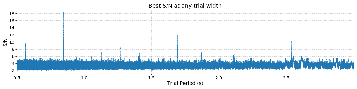
The fundamental period of the pulsar is visible along with a number of harmonics. Zooming in on the main peak we can fully appreciate the period resolution of the FFA:
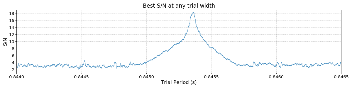
Peak Detection Algorithm
Periodogram peaks can be quickly and automatically found by riptide.find_peaks(). It returns a list of
peaks sorted by decreasing S/N, and a dictionary containing the polynomial coefficients of the
fitted selection threshold; the latter can be safely ignored except for very specific purposes.
>>> peaks, __ = find_peaks(pgram)
>>> main_peak = peaks[0]
>>> print(main_peak)

Peak(period=0.8453599547405023, freq=1.182928046676835, width=4, ducy=0.0163265306122449,
   iw=3, ip=114078, snr=18.23371124267578, dm=400.0)
Peak objects are python namedtuples. Here our pulsar is optimally detected at a trial
boxcar width of 4 bins and a period of 845.36 ms. It is important to note that the peak selection
threshold algorithm is applied to every trial width separately, which means that a
sufficiently bright signal will produce multiple peaks, up to one per trial width. This
significantly improves the detectability of narrow, long period pulsed signals; the topic is
discussed further Section 5 of the reference paper.
Making a sub-integrations plot
We can now fold the original data at the best detection period and have a look at the signal that we found:
bins = 512
subints = tseries_presto.fold(main_peak.period, bins, subints=64)

import matplotlib.pyplot as plt
plt.subplot(211)
plt.imshow(subints, cmap='Greys', aspect='auto')
plt.subplot(212)
plt.plot(subints.sum(axis=0))
plt.xlim(0, bins)
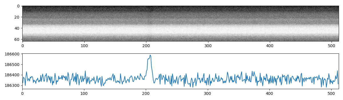
Not exactly what we might have expected. The data are dominated by red noise, but we can instead
fold the de-reddened version of the data produced (and searched) by ffa_search():
bins = 512
# This copy of the time series has been running median subtracted
subints = ts.fold(main_peak.period, bins, subints=64)

import matplotlib.pyplot as plt
plt.subplot(211)
plt.imshow(subints, cmap='Greys', aspect='auto')
plt.subplot(212)
plt.plot(subints.sum(axis=0))
plt.xlim(0, bins)
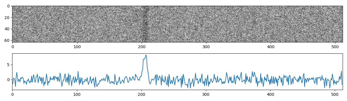
The pulsar signal now appears clearly, and has been visibly folded at the correct period.
The Metadata attribute
All TimeSeries objects and all derived data products (periodograms, pulsar search candidates,
etc.) in riptide have a Metadata dictionary carrying whatever information provided by the
software package that created the input time series data. There is no header standardization for
such data in pulsar astronomy, and the information contained in Metadata will therefore vary
across software packages and observatories. We do however attempt to guarantee some metadata
uniformity in riptide, by always enforcing the presence of the following metadata keys and their
associated data types:
dm:float, dispersion measure of the input datafname:str, original file namemjd:float, epoch of observationsource_name:strskycoord:astropy.SkyCoord, source coordinatestobs:float, integration time in seconds
If these required attributes were not provided by the original creator of the time series, they
are set to the special value None. Here’s the metadata for our TimeSeries of interest:
>>> print(tseries_presto.metadata)

{'analyst': 'vmorello',
'bandwidth': 400.0,
'barycentered': True,
'basename': 'J1855+0307_DM400.00',
'breaks': False,
'cbw': 0.390625,
'decj': '03:02:38.8000',
'dm': 400.0,
'fbot': 1182.1953125,
'fname': '/home/vince/work/time_series/J1855+0307/J1855+0307_DM400.00.inf',
'fov': 981.0,
'instrument': '????',
'mjd': 56937.40513572802,
'nchan': 1024,
'notes': 'Input filterbank samples have 2 bits.',
'nsamp': 8754411,
'observer': 'Unknown',
'obstype': 'Radio',
'raj': '18:55:04.4400',
'skycoord': <SkyCoord (ICRS): (ra, dec) in deg
   (283.7685, 3.04411111)>,
'source_name': 'G036.5+00.6_s',
'telescope': 'Parkes',
'tobs': 560.282304,
'tsamp': 6.4e-05}
The rseek command-line app
rseek is just a convenient way of searching a single DM trial from the command-line.
It loads the file, runs ffa_search(), gets the parameters of all significant periodogram peaks
with the find_peaks() function and prints them in a table. rseek does not save any
candidate files or data products; for more serious purposes, see Using the Pipeline.
Here’s an example using the same observation of PSR J1855+0307. We search a small range of periods
around that of the pulsar, which comes out as the top candidate followed by a number of harmonic
detections.
$ rseek --Pmin 0.5 --Pmax 2.0 --bmin 480 --bmax 520 -f presto J1855+0307_DM400.00.inf

     period          freq  width     ducy       dm    snr
0.845358133   1.182930596      9    1.81%   400.00   18.4
1.690716646   0.591465165      4    0.78%   400.00   12.9
0.563576780   1.774381123     13    2.61%   400.00    9.7
1.268034192   0.788622267      4    0.81%   400.00    8.6
1.869356204   0.534943526    141   29.19%   400.00    8.4
1.127147566   0.887195280      6    1.16%   400.00    7.7